more E1031 results

Here's an example of how the strip-hits simulated spectra results can be used. Take the results of different simulated reactions (for the one strip), add them together in different proportions to make a final combined spectrum, compare it with the data for that strip. Try:

all = 1*c13a + 0.2*c13p + 0.8*c12a + 0.05*c12p + 2.5*dp + 0.2*o16p + 1.5*o16a + 0.1*b11p + 0.1*b11a

where "c13a" is the alphas produced from reactions on ¹³C, and similarly for the other waves. Here's the results for the 19' strip.



The other thing to note is that the data energies have been shifted in this strip by
+12 channels * 10 keV/channel = +120 keV

Some of the synthetic peaks are good matches; others aren't. The thing is that these synthetic spectra populate all possible levels equally (taking no account of Jpi values or angular distributions). It would be interesting to make a plot that indicates only the locations of the peaks from various reactions, so that we could pick and choose which peaks from a given reaction are being populated.

...okay, here's what that would look like:

E1031 contaminant results

Simulation and data for 7.83 MeV 12C beam, 20 ug target: downstream LEDA innermost strip (19')



downstream LEDA outermost strip (41')

E1031 contaminant joy

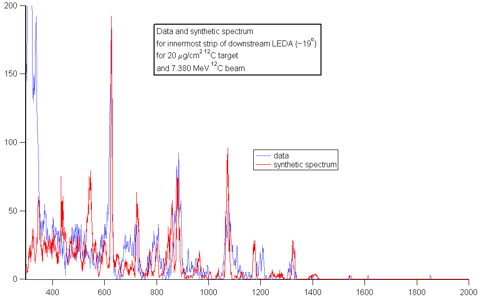
Goal: do simulations that give as output synthetic energy spectra for given strips of the current detector assembly. (I'd provide details of how the code produces the spectra, but Blogger keeps thinking that the java code is instructions on how to format the entry.) The code now cycles through all given excitation energies for a single reaction before producing two output files: one with all of the information and diagnostics for each event, and one with the combined energy hits in each strip for all excitation energies for that reaction.

Use the following inputs:
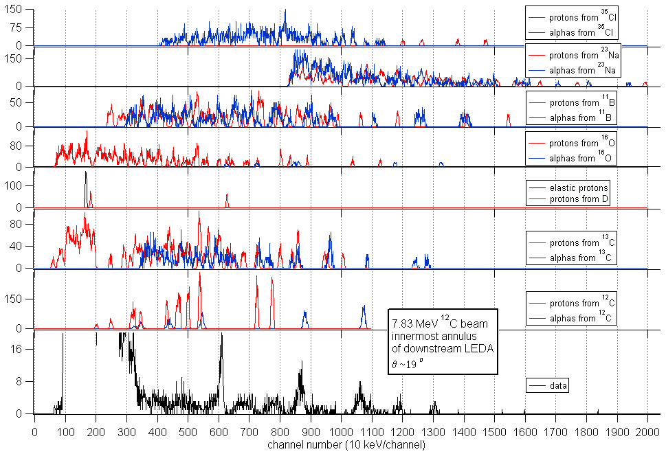
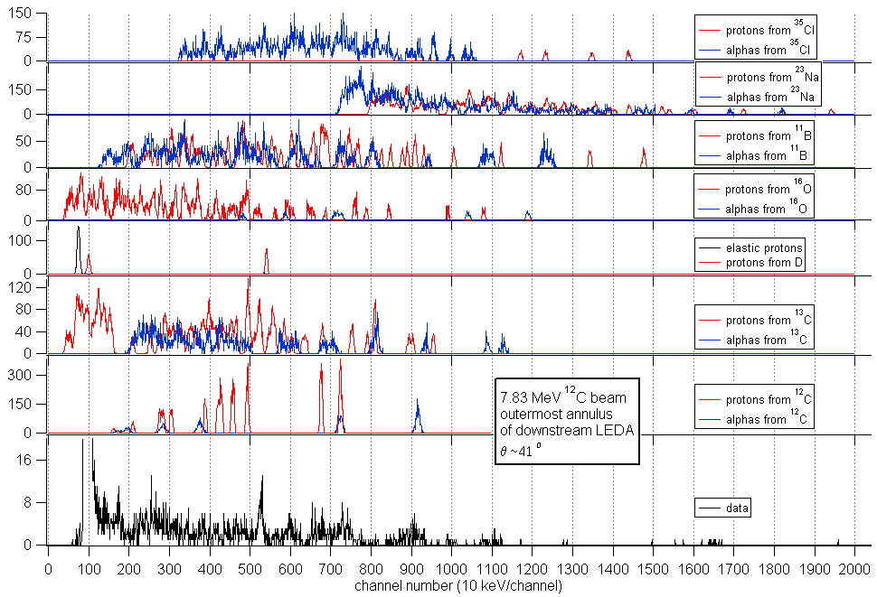
beam energy: 7.83 MeV
target: 20 μg/cm² C (for energy loss purposes)
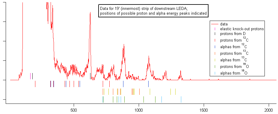
Reactions considered, with excitation energies of residual nucleus that result in outgoing particle energies between 1 and 20 MeV at 20':
¹²C(¹²C,p)²³Na (0-5.7 MeV)
¹²C(¹³C,p)²⁴Na (0-8)
¹²C(¹⁶O,p)²⁷Al (0-9)
¹²C(¹¹B,p)²²Ne (0-12.7)
¹²C(²³Na,p)³⁴S (0-17.6)
¹²C(³⁵Cl,p)⁴⁶Ti (0-13)
¹²C(p,p)¹²C (0)
¹²C(d,p)¹³C (0-3.3)
¹²C(¹²C,α)²⁰Ne (0-7)
¹²C(¹³C,α)²¹Ne (0-10)
¹²C(¹⁶O,α)²⁴Mg (0-10)
¹²C(¹¹B,α)¹⁹F (0-10)
¹²C(²³Na,α)³¹P (0-17)
¹²C(³⁵Cl,α)⁴³Sc (0-10)

Actual excitation energies used:
²³Na {0, 0.44, 2.076, 2.3907, 2.63986, 2.704, 2.982, 3.6776, 3.848, 3.914, 4.42963, 4.775}
²⁴Na {0, 0.472207, 0.5632, 1.34143, 1.34465, 1.34663, 1.5124, 1.84601, 1.88551, 2.51351, 2.5628, 2.90394, 2.97783, 3.2167, 3.37184, 3.41325, 3.58926, 3.62825, 3.65597, 3.68179, 3.74509, 3.896, 3.9357, 3.94339, 3.97732, 4.04849, 4.145, 4.1868, 4.1963, 4.20719, 4.22, 4.44154, 4.459, 4.526, 4.56206, 4.6215, 4.6922, 4.75094, 4.772, 4.89135, 4.9394, 4.98, 5.03, 5.0449, 5.05972, 5.11741, 5.16, 5.19244, 5.25, 5.33906, 5.39719, 5.432, 5.47896, 5.585, 5.6284, 5.66, 5.72, 5.774, 5.80966, 5.8629, 5.91846, 5.95316, 5.9662, 6.07283, 6.2224, 6.24762, 6.578, 6.96221, 6.96678, 6.99337, 7.01029, 7.0685, 7.072, 7.0858, 7.0966, 7.1416, 7.1513, 7.1631, 7.1862, 7.187, 7.1923, 7.2456, 7.2461, 7.2518, 7.3244, 7.3276, 7.3367, 7.3727, 7.3863, 7.4255, 7.4337, 7.4461, 7.4739, 7.4998, 7.5113, 7.519, 7.5323, 7.533, 7.6274, 7.6555, 7.708, 7.832, 7.903}
²⁷Al {0, 0.84376, 2.21201, 2.7349, 2.982, 3.0042, 3.6804, 3.9568, 4.0546, 4.4102, 4.5103, 4.58, 4.8116, 5.1556, 5.248, 5.4199, 5.4328, 5.4384, 5.4998, 5.5509, 5.6673, 5.7516, 5.827, 5.9603, 6.0808, 6.1158, 6.1584, 6.2847, 6.4628, 6.4773, 6.5122, 6.533, 6.6051, 6.6513, 6.713, 6.765, 6.7763, 6.8138, 6.8207, 6.9479, 6.9929, 6.996, 7.0713, 7.1736, 7.2272, 7.28, 7.289, 7.4, 7.413, 7.443, 7.4771, 7.55, 7.578, 7.66, 7.6765, 7.679, 7.721, 7.798, 7.806, 7.858, 7.9, 7.935, 7.948, 7.997, 8.037, 8.043, 8.065, 8.097, 8.13, 8.136, 8.1821, 8.287, 8.324, 8.361, 8.376, 8.396, 8.408, 8.4207, 8.442, 8.4903, 8.521, 8.537, 8.553, 8.586, 8.5976, 8.675, 8.693, 8.7087, 8.7166, 8.7322, 8.7536, 8.7742, 8.804, 8.825, 8.861, 8.8972, 8.905, 8.9092, 8.952, 8.9634, 9.001}
²²Ne {0, 1.274542, 3.3582, 4.4563, 5.1463, 5.329, 5.3634, 5.5237, 5.6414, 5.9099, 6.1199, 6.235, 6.3111, 6.3452, 6.6358, 6.691, 6.8194, 6.8535, 6.9, 7.051, 7.3411, 7.3437, 7.4059, 7.423, 7.469, 7.489, 7.6431, 7.664, 7.722, 7.921, 8.0769, 8.1343, 8.1622, 8.3759, 8.4896, 8.5614, 8.596, 8.741, 8.8553, 8.9003, 8.976, 9.045, 9.097, 9.178, 9.1781, 9.229, 9.25, 9.324, 9.508, 9.541, 9.652, 9.725, 9.842, 10.066, 10.137, 10.2089, 10.2808, 10.2953, 10.384, 10.423, 10.469, 10.4933, 10.618, 10.696, 10.706, 10.751, 10.858, 10.922, 11.032, 11.13, 11.195, 11.271, 11.433, 11.466, 11.52}
³⁴S {0, 2.127564, 3.304212, 3.91641, 4.074667, 4.11481, 4.624404, 4.68898, 4.87684, 4.88976, 5.22818, 5.32251, 5.38099, 5.679927, 5.689, 5.75588, 5.84753, 5.9981, 6.12148, 6.16886, 6.25122, 6.25168, 6.34249, 6.42142, 6.42812, 6.47877, 6.535, 6.639, 6.68533, 6.729, 6.742, 6.82882, 6.84791, 6.8637, 6.89, 6.95422, 7.11045, 7.16446, 7.21928, 7.24805, 7.27, 7.36742, 7.392, 7.46772, 7.55269, 7.62991, 7.657, 7.714, 7.73079, 7.753, 7.78122, 7.788, 7.795, 7.97472, 8.02, 8.0363, 8.083, 8.1381, 8.1751, 8.18546, 8.2054, 8.255, 8.264, 8.293, 8.29439, 8.369, 8.3854, 8.425, 8.502, 8.50677, 8.61574, 8.651, 8.657, 8.67, 8.70235, 8.712, 8.72763, 8.733, 8.782, 8.8057, 8.87402, 8.876, 8.942, 8.968, 8.99, 9.02631, 9.095, 9.15871, 9.20804, 9.478, 9.54609, 9.59841, 9.64, 9.66574, 9.711, 9.80188, 9.8367, 9.86, 9.93335, 9.981, 10.09221, 10.097, 10.142, 10.17, 10.17, 10.17959, 10.201, 10.21215, 10.237, 10.25, 10.31153, 10.386, 10.407, 10.447, 10.494, 10.529, 10.587, 10.617, 10.626, 10.6501, 10.663, 10.67, 10.705, 10.768, 10.791, 10.803, 10.84062, 10.869, 10.895, 10.916, 10.931, 10.994, 11.015, 11.02494}
⁴⁶Ti {0, 0.889286, 2.009846, 2.611, 2.9618, 3.05846, 3.168, 3.213, 3.2173, 3.2357, 3.29886, 3.338, 3.44139, 3.5531, 3.5693, 3.5717, 3.5798, 3.6102, 3.677, 3.696, 3.7238, 3.731, 3.7379, 3.7715, 3.82643, 3.845, 3.848, 3.85244, 3.856, 3.872, 3.8893, 3.9056, 3.926, 3.9419, 4.0031, 4.0253, 4.0388, 4.1301, 4.1787, 4.1915, 4.3158, 4.3226, 4.372, 4.398, 4.4171, 4.437, 4.5, 4.5234, 4.527, 4.573, 4.617, 4.6623, 4.675, 4.697, 4.7264, 4.791, 4.8272, 4.845, 4.8969, 4.95, 5, 5.0237, 5.079, 5.094, 5.117, 5.154, 5.18, 5.1976, 5.206, 5.23, 5.28, 5.321, 5.361, 5.363, 5.409, 5.515, 5.53, 5.604, 5.61, 5.7, 5.794, 5.811, 5.828, 5.84, 5.872, 5.903, 5.95, 5.965, 5.992, 6.021, 6.025, 6.094, 6.118, 6.134, 6.1505, 6.2004, 6.217, 6.2419, 6.251, 6.266, 6.305, 6.338, 6.36, 6.395, 6.398, 6.424, 6.458, 6.513, 6.55, 6.574, 6.616, 6.685, 6.739, 6.794, 6.8303, 6.851, 6.89, 6.958, 6.974, 7.019, 7.041, 7.101, 7.12, 7.147, 7.172, 7.18, 7.201, 7.238, 7.288, 7.312, 7.35, 7.392, 7.41, 7.429, 7.472, 7.534, 7.558, 7.584, 7.608, 7.63, 7.66, 7.71, 7.73, 7.735, 7.788, 7.849, 7.874, 7.917, 7.937, 7.9418, 7.9608, 7.979, 8.013, 8.02, 8.04, 8.088, 8.134, 8.182, 8.2175, 8.23, 8.2839, 8.293, 8.346, 8.384, 8.46, 8.467, 8.53, 8.574, 8.621, 8.662, 8.701, 8.7162, 8.761, 8.808, 8.86, 8.94, 8.984, 9, 9.07, 9.111, 9.141, 9.168, 9.17, 9.205, 9.253, 9.304, 9.345, 9.399, 9.42, 9.426, 9.474, 9.519, 9.55, 9.572, 9.615, 9.649, 9.67, 9.682, 9.718, 9.761, 9.77, 9.79, 9.852, 9.864, 9.87, 9.973, 10, 10.038, 10.0416, 10.18, 10.212, 10.256, 10.321, 10.347, 10.35, 10.374, 10.38, 10.441, 10.523, 10.602, 10.661, 10.73, 10.782, 10.866, 10.938, 10.98, 11.05, 11.051, 11.11, 11.167, 11.299, 11.354, 11.3742, 11.426, 11.45, 11.57, 11.698, 11.84, 12.2, 12.46, 12.65, 12.974}
¹²C {0}
¹³C {0.0,3.089}
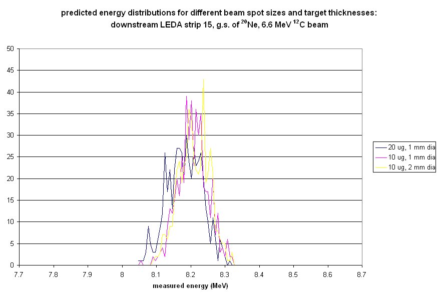
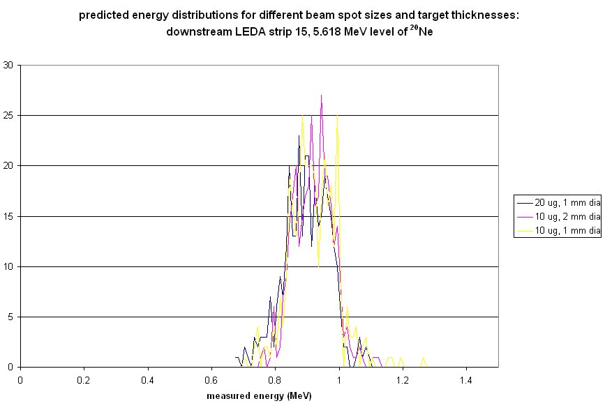
²⁰Ne {0, 1.633674, 4.2477, 4.96651, 5.6214, 5.7877}
²¹Ne {0, 0.350727, 1.745911, 2.78823, 2.79416, 2.8666, 3.66264, 3.73559, 3.88396, 4.4318, 4.52586, 4.68456, 4.72534, 5.3352, 5.4318, 5.5498, 5.6308, 5.68977, 5.7737, 5.8187, 5.8209, 5.99261, 6.0333, 6.1752, 6.2603, 6.2667, 6.4119, 6.4483, 6.5435, 6.5542, 6.6077, 6.6398, 6.7493, 6.857, 6.9005, 7.0067, 7.0226, 7.0421, 7.109, 7.154, 7.211, 7.226, 7.294, 7.32, 7.3569, 7.4228, 7.465, 7.547, 7.6, 7.627, 7.6491, 7.74, 7.81, 7.9603, 7.979, 7.9821, 8.008, 8.062, 8.1549, 8.2222, 8.2412, 8.287, 8.303, 8.36, 8.402, 8.43, 8.465, 8.522, 8.591, 8.6645, 8.68, 8.782, 8.801, 8.849, 8.8592, 8.93, 8.991, 9.077, 9.1489, 9.188, 9.251, 9.282, 9.367, 9.402, 9.475, 9.637, 9.7, 9.8591, 9.9436, 9.963}
²⁴Mg {0, 1.368675, 4.122874, 4.23836, 5.2352, 6.01032, 6.4325, 7.34905, 7.5553, 7.61647, 7.7477, 7.8122, 8.113, 8.3581, 8.4384, 8.4393, 8.6549, 8.8645, 9.0035, 9.1462, 9.2844, 9.2998, 9.30095, 9.3054, 9.4578, 9.51621, 9.528, 9.5327, 9.8284, 9.9678}
¹⁹F {0, 0.109894, 0.197143, 1.34567, 1.4587, 1.554038, 2.779849, 3.90817, 3.9987, 4.0325, 4.3777, 4.5499, 4.5561, 4.648, 4.6825, 5.1066, 5.337, 5.418, 5.4635, 5.5007, 5.535, 5.621, 5.938, 6.07, 6.088, 6.1, 6.1606, 6.255, 6.282, 6.33, 6.429, 6.4967, 6.5, 6.5275, 6.554, 6.592, 6.787, 6.8384, 6.891, 6.9265, 6.989, 7.114, 7.1662, 7.262, 7.364, 7.5396, 7.56, 7.587, 7.6606, 7.702, 7.74, 7.9, 7.929, 7.937, 8.014, 8.084, 8.1377, 8.16, 8.199, 8.2543, 8.288, 8.31, 8.37, 8.5835, 8.5919, 8.629, 8.65, 8.7932, 8.864, 8.9267, 8.953, 9.03, 9.0997, 9.101, 9.167, 9.204, 9.267, 9.28, 9.318, 9.321, 9.329, 9.509, 9.527, 9.5364, 9.566, 9.575, 9.586, 9.642, 9.654, 9.6675, 9.71, 9.82, 9.834, 9.874, 9.887, 9.895, 9.926}
³¹P {0, 1.26615, 2.2337, 3.1341, 3.295, 3.4146, 3.5058, 4.1903, 4.2607, 4.4309, 4.5936, 4.6338, 4.7831, 5.0149, 5.0152, 5.1154, 5.2561, 5.3431, 5.5293, 5.5592, 5.6723, 5.7731, 5.8923, 5.9879, 6.0478, 6.0801, 6.2331, 6.3366, 6.3808, 6.3986, 6.4537, 6.4608, 6.4958, 6.5006, 6.5942, 6.6103, 6.7929, 6.8251, 6.8423, 6.9092, 6.9317, 7.068, 7.0799, 7.084, 7.1179, 7.1406, 7.214, 7.3137, 7.3144, 7.349, 7.4412, 7.466, 7.687, 7.715, 7.736, 7.7793, 7.825, 7.852, 7.8968, 7.913, 7.9455, 7.994, 8.0322, 8.0487, 8.085, 8.1047, 8.208, 8.2247, 8.243, 8.2471, 8.3455, 8.3556, 8.4338, 8.4609, 8.4702, 8.5435, 8.5521, 8.5553, 8.5755, 8.584, 8.6008, 8.6411, 8.6493, 8.7289, 8.7304, 8.7378, 8.7541, 8.7572, 8.7632, 8.8398, 8.9028, 8.9096, 8.9357, 8.9857, 9.0089, 9.046, 9.0526, 9.067, 9.1134, 9.1155, 9.1285, 9.1309, 9.1542, 9.1563, 9.176, 9.2061, 9.2263, 9.2407, 9.2529, 9.2559, 9.2908, 9.3196, 9.3582, 9.3609, 9.3624, 9.3998, 9.4125, 9.4408, 9.4489, 9.477, 9.524, 9.5247, 9.534, 9.5365, 9.5705, 9.5778, 9.5805, 9.5851, 9.5939, 9.5985, 9.6119, 9.659, 9.7205, 9.7228, 9.756, 9.76, 9.765, 9.765, 9.787, 9.814, 9.816, 9.819, 9.84, 9.843, 9.852, 9.865, 9.867, 9.907, 9.908, 9.925, 9.928, 9.941, 9.946, 9.963, 9.976, 9.988, 9.999, 10.017, 10.019, 10.046, 10.075, 10.089, 10.092, 10.093, 10.098, 10.116, 10.144, 10.153, 10.192, 10.207, 10.21, 10.225}
⁴³Sc {0, 0.1514, 0.4723, 0.8452, 0.8551, 0.8803, 1.1584, 1.1789, 1.3368, 1.408, 1.6508, 1.8107, 1.8299, 1.8826, 1.9314, 1.9629, 2.0943, 2.106, 2.1143, 2.1417, 2.2426, 2.2883, 2.3354, 2.3827, 2.4586, 2.5525, 2.58, 2.6354, 2.657, 2.6703, 2.76, 2.7952, 2.8107, 2.84, 2.8462, 2.861, 2.875, 2.93, 2.9849, 2.9874, 3.1232, 3.1406, 3.1588, 3.1976, 3.2598, 3.2929, 3.3272, 3.332, 3.3752, 3.4515, 3.4633, 3.48, 3.503, 3.613, 3.6315, 3.6454, 3.683, 3.7, 3.7338, 3.7547, 3.757, 3.8066, 3.843, 3.86, 3.894, 3.939, 3.949, 4.007, 4.038, 4.138, 4.157, 4.211, 4.236, 4.276, 4.36, 4.371, 4.382, 4.43, 4.455, 4.511, 4.555, 4.584, 4.665, 4.7, 4.72, 4.766, 4.817, 4.875, 4.895, 4.942, 5.022, 5.187, 5.2, 5.236, 5.262, 5.327, 5.461, 5.49, 5.5173, 5.53, 5.641, 5.72, 5.822, 5.871, 5.919, 5.976, 6.032, 6.079, 6.105, 6.143, 6.217, 6.282, 6.384, 6.4287, 6.444, 6.685, 6.696, 6.71, 6.811, 6.917, 7.3549}

Orsay: elastic scattering efficiency

Just realized I haven't shared pictures of the detection efficiency from the elastic scattering sims: total number of hits with configurations A B C...


...and fractional efficiency per angular bin...


Like I said before, config C isn't all that different from A or B for the elastic scattering: where it really improves the efficiency is for the reaction.

yet another comment on Orsay: beam spot size

All the simulations below assume a 1-mm diameter beam spot. The width of the Q-value distributions is actually quite sensitive to beam spot size. I won't taunt you by showing plots of what the resolution would look like if the beam were on axis, but here's what the two states in ¹⁸O look like for a 2-mm diameter beam spot:



The widths of the peaks are now 63 keV instead of 51 keV for the 1 mm diameter beam spot, so worse but not catastrophic.

further note on the Orsay sims: threshold and "good events"

The PSSSD detectors have energy thresholds on both ends of each strip. The threshold is set to 500 keV right now. What that looks like in the code:

TflightResid = energy of ¹⁸O after dead layer of detector
RX0 = x-position of ¹⁸O along detector strip
...and the length of a detector is 50 mm, so the energy measured in either end is ERA or ELA:

ERA=TflightResid *(RX0+25)/50;
ELA=TflightResid-ERA;
if ((ELA >= hit_threshold)&&(ERA >= hit_threshold)) energyHitA=true;

...also: the Q-value distributions are made only from "good events": the ¹⁸O hits one of the "single" PSSSD detectors, and both alphas hit both a dE pad detector and the matching E PSSSD detector. There's a lot more events in the simulations that don't meet all those criteria.

details of Orsay Q-value calculation

Ebeam = initial beam energy (80 MeV)
Tbeam = real T of beam just before reaction
TinitResid = initial energy of ¹⁸O
TinitPF1,2 = initial alpha energies
Tflight... = energy after passing through target, dead layer of E detector, and poss. dE detector

double Qtrue=-(Tbeam-TinitResid-TinitPF1-TinitPF2); //this is the real god-given Q value of the reaction
double px=Math.sqrt(2*beam.A*Ebeam);//"x" is direction of beam
double p1=Math.sqrt(2*projfrag.A*TflightPF1);
double p2=Math.sqrt(2*projfrag.A*TflightPF2);
double px1=p1*Math.cos(Math.toRadians(thetaCalc1));
double px2=p2*Math.cos(Math.toRadians(thetaCalc2));
double py1=p1*Math.sin(Math.toRadians(thetaCalc1));
double py2=p2*Math.sin(Math.toRadians(thetaCalc2));
double pxresid=px-px1-px2;
double pyresid=py1+py2;
double Eresid=(pxresid*pxresid+pyresid*pyresid)/(2*18);//the residual will always be assumed to be ¹⁸O; for contaminants, it will obviously be something else really, but this is the Q-value we'll get
double Qcalc = -(Ebeam-TflightPF1-TflightPF2-Eresid); // this is the best way of calculating the Q value
double Qcalc2 = -(Ebeam-TflightPF1-TflightPF2-TflightResid); // using the measured ¹⁸O energy gives worse resolution

more on contaminants

...with more levels and with ²⁰Ne:





It looks like the kinematics will let us separate out the ¹⁶O reaction products, so they shouldn't be a problem for the Q-value calculation, and there are no natural-parity levels in ¹⁹O between the 5.7046 and 6.1196 MeV levels that were simulated--and those ones give Q values just to either side of the 6.404 MeV ¹⁸O peak of interest, so the ¹³C contamination shouldn't be a problem either.

woohoo!

Preliminary contaminant results: Orsay

In words: ¹³C + ¹⁴C --> ¹⁹O + 2 alpha with ¹⁹O Ex=5.5 MeV could probably be confused with ¹⁸O Ex=6.4 MeV, just by the energy vs. theta for the heavy ion tag, but the Q values calculated for both are different enough that we can cleanly separate those states.

Orsay results: effect of target thickness and Q calculation method on resolution

(Everything here assumes the detector configuration C discussed below, and a 1 mm diameter beam spot.)
First, use 10 μg/cm² target, and compare different ways of calculating the Q-value: use the measured energies for both alphas and the ¹⁸O, and also deduce the ¹⁸O energy from the measured alpha energies. results:

It's clearly better to just use ¹⁸O as a tag, and not attach any significance to its measured energy, since it's subject to a lot of energy loss/straggling in the target (even at 10 μg/cm²). All cool.

Now compare two target thicknesses: 10 μg/cm² and 100 μg/cm². Use the alphas-only Q-value calculation method. results:

What that says to me is that even at 100 μg/cm² it should be possible to see the presence of the 6.351 MeV level: the difference in energies/Q values is about 55 keV, and at 100 μg/cm² the peak width is about 51 keV (while at 10 μg/cm² it's only about 30 keV)--so if the 6.351 MeV level is populated, it will either produce a tail on the 6.404 peak or will broaden it noticeably.

Comments? Thoughts?

Coming up next: Contaminants!

Orsay: srimulations and Ex + Jpi

In our last exciting episode, we learned about different detector configurations and how they affect our total detection efficiency. This time we'll learn about the energy resolution of the detectors. Can our intrepid hero(in)es see the effect of the extra level, or are they doomed to not be able to resolve it? Stay tuned.

------------------

Srimulations:
beam in target:
double EStraggleEntrance = 0.2*targetLoss*random.nextGaussian()/2.35;
double angStraggleBeamEntrance = 0.03*random.nextGaussian()*xtarg/(100*2.35);
double ThetaBeam = Math.abs(0.03+angStraggleBeamEntrance);

¹⁸O in target: srimulated 8 MeV, since these are about the lowest energy produced in the relevant angular range
double EStraggleResidTarget = 0.04*residualTargetLoss*random.nextGaussian()/2.35;
thetaResidLab = thetaResidLab+0.7*random.nextGaussian()*xtarg/(100*2.35);

alpha in target: srimulated 10 and 1 MeV
double EStraggleTarget=0.33*a1TargetLoss*random.nextGaussian()/2.35;
thetaDlabPF1=thetaDlabPF1+0.12*random.nextGaussian()*xtarg/(100*2.35);

alpha in delta-E detector: srimulated 30,20,15,10 MeV in 60 um of Si
DELoss1 = DELossCalc.getThinEnergyLoss(projfrag,TflightPF1,PF1ThetaInc) *(0.001+0.00007*random.nextGaussian()/2.35);
double fwhm=0.5;
if (DELoss1>2.5) fwhm=DELoss1-2;
double angStraggleDE1=fwhm*random.nextGaussian()/2.35;

srimulated 7, 14, 30, 60 MeV 18O in dead layer of X2 detectors; in all cases, the energy loss fwhm was 0.08 MeV (!).

checked energy loss in various absorbers:

• the beam energy loss in the target looks the same in the simulation as in the SRIMulation.
  
• The dead layer parameters were copied from the E1031 sims.
  
• The alpha energy loss in the pad detector is the same at 20 MeV, but greater for lower energy. This is the dedx vs srim issue again. I don't know how to fix it properly...but it is important to have the right energy loss in the pad detectors, since we use the alpha energies to calculate the Q value.... How about this: for energies above 20 MeV, use the energy loss the simulation would normally calculate, but below 20 MeV use an energy dependent function...
  

(this is filler text to thwart the evil computer.)

double mod2=1;
if (TflightPF2<20) mod2=0.77+0.0115*TflightPF2; deloss2=0.001*mod2*DELossCalc.getThinEnergyLoss(projfrag,TflightPF2,PF2ThetaInc);
destrag2=0.055*DELoss2*random.nextGaussian()/2.35;

(this is filler text to thwart the evil computer.)

That energy dependence makes the simulation's result match SRIM's. all is well.

------------------

Allowed Jpi values: Jpi selection rules



i.e. for small angular momentum transfers, 0+,1-,2+,... levels in ¹⁸O will be populated; same thing in ²²Ne (from reactions on 16O contaminant); and in ¹⁹O (from reactions on ¹³C contaminant) the 1/2-, 3/2+, 5/2-... levels will be populated.

The ¹⁸O level of interest (6.404 MeV) has Jpi=3-. The potential contaminant (6.351 MeV) is thought to have Jpi=2-. If this is the correct Jpi assignment, the level won't be populated--but the assignment might be incorrect so I'll simulate its effect anyway.

In ²²Ne, there are natural parity levels at:
Ex (MeV) Jpi
0 0+
1.275 2+
3.3577 4+
4.4558 2+
5.3632 2+
5.5237 4+
5.9101 3-
6.1201 2+
6.2343 0+
63103 6+
6.3465 4+
6.691 1-
6.8194 2+
6.9003 (0,1)+
7.0509 1-
7.3407 0+
7.3428 (3,4)+
7.4059 3-
7.469 ?
7.491 1-
7.6430 2+
7.722 3-
7.9226 (2)+
8.0764 (4)+
8.1343 2+
8.1618 2+,3,4+
8.3759 (3)-
8.452 ?
8.4887 2+
8.553 (1,2)+
8.573 ?
8.5960 2+
8.7400 (3)-
8.8549 4+
8.8990 ?
8.976 ?
9.045 2+,3-
9.097 1-
9.162 ?
9.1775 (4)+
9.229 2+
9.250 ?
9.324 ?
9.508 ?
9.541 2+
9.625 ?
9.652 ?
9.725 (3-)
9.842 (2+)

and in ¹⁹O, the natural parity levels are at
Ex (MeV) Jpi
0.0960 3/2+
2.7790 7/2+
3.0674 3/2+
3.2316 (1/2, 3/2-)
4.1093 3/2+
4.3281 3/2, 5/2
4.4025 3/2, 5/2, 7/2
4.9683 5/2, 7/2
5.0070 3/2, 5/2
5.0820 1/2-
5.1484 >=5/2+
5.3840 9/2, 11/2, 13/2
5.5035 ?
5.540 3/2+
5.7046 7/2-, 5/2
6.1196 3/2+
6.1916 ?
6.4058 ?
6.4662 7/2, 9/2, 11/2
6.583 ?
6.903 ?
6.988 ?

new blog template!

The links that used to be in the sidebar are now at the bottom of the page. The sidebar was eating up too much of the page width and annoying me. Besides, physicists don't DO coloured backgrounds, do they? No, no they don't.

note about S2s in E1031

In all the simulations I've done so far, I've left out the upstream S2s since they were eventually switched off after being clobbered by beam last July. There's probably still some good information there, so eventually I'll need to simulate them too.

E1031 alpha calibration

Here's what the real measured energies from the triple alpha source look like in TUDA as used in July.
geometry:
upstream LEDA is 45 mm from the target
downstream LEDA is 150 mm "
(downstream) S2 is 170 mm "
dead layers: 0.33 um for LEDA, 0.39 um for S2: explained in the previous entry: these are the values I needed to reproduce the SRIM results for 0.4 and 0.8 um respectively.



(A note about the figure: the blue points are the actual values for individual alpha events. The pink points are a clever way of using those values in the code to automatically calculate average energies and angles for each strip...except that as you can see they don't always give the right values for the average energies. I have absolutely no idea why this is so, and particularly why it's only the S2 energy where this problem shows up. However, the LEDA values seem to agree well with the actual averages for each strip, so I've used those automatically-calculated averages below to calculate E(alpha) as a function of strip number.)

For the downstream Leda and the S2, the angle dependence isn't too bad, but for the upstream Leda it is. I suggest using the following linear fits:
For downstream LEDA:
"5.155 MeV" energy = -0.001144 * strip number + 5.0871
"5.486 MeV" energy = -0.001047 * strip number + 5.4211
"5.806 MeV" energy = -0.000988 * strip number + 5.7440
For upstream LEDA:
"5.155 MeV" energy = -0.006499 * strip number + 5.0563
"5.486 MeV" energy = -0.006187 * strip number + 5.3923
"5.806 MeV" energy = -0.005906 * strip number + 5.7168
and for S2:
"5.155 MeV" energy = 5.0089
"5.486 MeV" energy = 5.3475
"5.806 MeV" energy = 5.6741

A note on LEDA strip numbering: the strip numbers are calculated here as
DLstrip=(int)Math.floor((rDL-50)/5);
that is, the numbering goes from the inner radius to the outer radius. I'm pretty sure this is the opposite from the numbering in the actual data, but it'll be easy to convert.
Update: weird. It turns out the numbering is the same in the simulation as in the data. How'd that happen? I must have checked the data analysis code when I was writing the simulation code, or something crazy like that. Anyway, in the simulation the distance from the beamline is defined as
DLrad=5*DLstrip+52.5;
whereas in the data analysis code it's
leda1_y = 5.25 + ledastrip1*0.5 (plus a randomizing factor)
which is the same, except for the change of units from mm to cm.

dirty secrets about absorber thickness

SRIM results for 5.486 MeV He passing through S2 or LEDA dead layer:
S2: 0.8 um Al, average angle 10', average energy loss 126 keV.
LEDA: 0.4 um Al, average angle 30', average energy loss 72 keV.

The java code gives 233 keV loss through the S2, for alphas of the same energy. This is something I've run into before: the parameters used to calculate energy losses (from Ziegler's tables--I think they're the same as in the DEDX code) are usually pretty close to SRIM, but sometimes differences do show up. An inelegant way around this problem is to enter a fake thickness for the dead layer, chosen so that the java code's energy loss for that thickness matches SRIM's energy loss for the real thickness.

So far I've been using 108 ug/cm2 = 0.4 um for LEDA's dead layer thickness, and twice that for the S2. The values that give sensible answers are 88 ug/cm2=0.33 um for LEDA and 106 ug/cm2 = 0.39 um for S2. These are what I used in the alpha calibration simulation.

note to self: backward angles

--make sure energy loss calculations use the angle through the material, not the angle in the lab. This was correct in the target for the most recent batch of triumf sims but incorrect for the upstream LEDA deadlayer calculation.

Tomas el Sabio would never make a mistake like that.

acronym JOY

TUDA = Tom's Under Duress Again

...also:

TDC Use Demands Attention

Torment Us Do Amplifiers

TUDA Users Demand Alcohol

TRIUMF 12C+12C simulation results: target thickness, beam spot size, angular distribution

Angular distributions of reaction protons and alphas, for last july's set-up:

energy distribution for alphas from ground state of ²⁰Ne:

...and for Ex=5.618 MeV:


What those energy distributions suggest is that it doesn't affect the energy resolution if we use 20 ug/cm² targets instead of 10 ug; also that the beam spot size isn't something to worry about. (these simulations don't take into account the incoming angle of the beam, which would be worsened by making the spot size smaller.)

SRIMulation JOY! (mostly for E1031 but possibly generally useful)

5 MeV 12C in 20 ug/cm2 12C at 0': E fwhm=12% DE; dtheta =0.2, fwhm=0.2
5 MeV 12C in 20 ug/cm2 12C at 10': E fwhm=13% DE; dtheta fwhm=0.3
8 MeV 12C in 20 ug/cm2 12C at 10': E fwhm=15% DE; dtheta fwhm=0.2
--> for the beam energy loss in the target for the triumf 12C+12C experiment, use the following code:

double beamStraggle = 0.15*targetLoss*random.nextGaussian()/2.35;
double thetaBeam = (depth/20)*(0.3 + 0.3*random.nextGaussian()/2.35);

He E de fwhm % dtheta fwhm
12 70% 0.02
5 39% 0.1
1 17% 0.5
0.5 17% 1
= 0.05E + 0.14 = -0.16x + 0.9
H E de fwhm % dtheta fwhm
8 157% 0.02
4 126% 0.06
1 71% 0.2
0.5 49% 0.5
= 0.14E + 0.5 = -0.1x + 0.4

(and no, I don't expect that table to mean anything to anyone except me.)
so for He in target use

double ejectileEStrag = (Tinit*0.05 + 0.14)*ejectileTargetLoss *random.nextGaussian()/2.35;
thetaDlab = thetaDlab + (0.9-0.16*Tinit)*(depthEjectile/20) *random.nextGaussian()/2.35;
if (Tinit>5) thetaDlab = thetaDlab + 0.02*(depthEjectile/20) *random.nextGaussian()/2.35;

and for H in target use

double ejectileEStrag = (Tinit*0.14 + 0.5)*ejectileTargetLoss *random.nextGaussian()/2.35;
thetaDlab = thetaDlab + (0.4-0.1*Tinit)*(depthEjectile/20) *random.nextGaussian()/2.35;
if (Tinit>4) thetaDlab = thetaDlab + 0.02*(depthEjectile/20) *random.nextGaussian()/2.35;

E	He shield de fwhm %	He shield dtheta fwhm
10	6%	0.75
5.1	5%	2.6
3.5	5%	6.4
	y=6%	y = -2x + 15
E	He dl de fwhm %
10	26%
3	11%
0.9	8%
	y = 0.02x + 0.06
E	H shield de fwhm %	H shield dtheta fwhm
10	33%	0.32
3	12%	1.2
1	12%	8
	y = 0.03x + 0.07	y = -3x + 11
E	H dl de fwhm %
10	107%
3	59%
1	27%
	y=0.08x+0.3

for He in shield use

EStraggleShield = 0.06*shieldLoss*random.nextGaussian()/2.35;
thetaDlabAl= thetaDlab + (15-2*Tflight)*random.nextGaussian()/2.35;
if (Tflight>6) thetaDlabAl= thetaDlab + 0.75*random.nextGaussian()/2.35;

for He in dead layer (LEDA or other detectors) use

EStraggleDead = (Tflight2*0.02 + 0.06)*deadlayerLoss*random.nextGaussian()/2.35;

for H in shield use

EStraggleShield = (Tflight*0.03 + 0.07)*shieldLoss*random.nextGaussian()/2.35;
thetaDlabAl= thetaDlab + (11-3*Tflight)*random.nextGaussian()/2.35;
if (Tflight>4) thetaDlabAl= thetaDlab + 0.4*random.nextGaussian()/2.35;

for H in dead layer (LEDA or other detectors) use

EStraggleDead = (Tflight2*0.08 + 0.3)*deadlayerLoss*random.nextGaussian()/2.35;

simulations for 12C+12C TRIUMF experiment

(more joy to follow)

Orsay detector geometry

The experiment: 80 MeV ¹⁴C on a ¹²C target-->¹⁸O+ ⁸Be. We detect the ¹⁸O and two alpha particles from the break-up of the ⁸Be.

The question: When we're measuring the 6.404 MeV level in ¹⁸O, does the 6.351 MeV level (if it's populated) add to the width in a measurable way? Do we need to use a thin target to see this contribution to the width? What about contaminants from ¹³C, ¹⁶O--can they be eliminated?

The kinematics: (click on any image to see a larger version, i.e. one in which the text is legible.)

Note that the maximum angle for ¹⁸O is 34', so there's no point putting detectors at high angles if they're just meant to be measuring ¹⁸O. Also, this plot shows the angle of the ⁸Be, but we measure its decay products: two alpha particles. We assume that the break-up occurs before the ⁸Be loses any energy in the target.

The detectors: a bunch of Micron X2 position sensitive silicon strip detectors, plus some 60 ug "pad" delta-E detectors. The initial proposal for the detector configuration is as follows...

It was also suggested to use out-of-plane detectors, in pairs or singly. I tried a bunch of different detector configurations.
Option A:
rd={250,170,170,250,170,170,240,160,160};
thetad={10,15,34,10,15,34,10,15,34};
phid={90.1,0.1,0.1,270.1,180.1,180.1,90.1,0.1,0.1};
Option B:
rd={250,250,170,250,250,170,240,240,160};
thetad={10,23,15,10,23,15,10,23,15};
phid={90.1,90.1,0.1,270.1,270.1,180.1,90.1,90.1,0.1};
Option C:
rd={170,210,210,170,210,210,160,200,200};
thetad={16,11,26,16,11,26,16,11,26};
phid={90.1,0.1,0.1,270.1,180.1,180.1,90.1,0.1,0.1};
(this was the input my simulation took. I don't understand why it was necessary to use 0.1 instead of 0, but it was.)
rd[i] is the radial distance of detector i from the target. thetad[i] and phid[i] are its angles. (The positive-z axis is the downstream beam direction and the x axis is horizontal.) Each detector is oriented so that its normal points to the target. (Makes calculations simple and also minimizes the dead layer effects.) Theta determines whether the detector is forward or backward; Phi determines whether the detector is in plane (0,180) or out of plane (90,270). In configs A and B, I was trying to get the in-plane detectors as close as possible and then fitting in the out-of-plane detectors at positions where they wouldn't be blocked; for config C I tried to make the radial distances pretty much the same for all detectors. (The dE detectors, i=6,7,8, are all set forward 1 cm from their corresponding E detectors, i=0,1,2.)
I tested the efficiency of each configuration using both elastic scattering and the reaction itself. For elastic scattering I used a cross section that was like the Rutherford cross section, normalized to the cross section at 8'. (For each event, a direction was randomly generated, its cross section was calculated, another random number [0,1] was generated, and the direction was accepted if the random number was less than the cross section.) For the reaction, the cross section was calculated from the centre-of-mass angle of the ⁸Be, using a parametrized fit to Kelly's Fresco calculations: 20*exp(-0.1*theta cm in degrees). This gives values from 11 mb/sr at 6' to 0.1 mb/sr at 51'.
The following figures show the efficiency of the three configurations for detecting elastic scattering.
Config A:

Config B:

Config C:

The efficiency numbers are as follows...
Config A
elastic hits
det 0 697
det 1 577
det 2 13
det 3 678
det 4 536
det 5 11
total 2512

reaction hits
dets 3,6 97
dets 4,7 149
dets 5,8 14
not 3,6 290
not 4,7 114
not 5,8 290
total hits 395

Config B

elastic hits
det 0 715
det 1 26
det 2 540
det 3 705
det 4 27
det 5 557
total 2570

reaction hits
dets 3,6 95
dets 4,7 0
dets 5,8 160
not 3,6 160
not 4,7 264
not 5,8 229
total hits 395

Config C:
elastic hits
det 0 407
det 1 804
det 2 21
det 3 433
det 4 812
det 5 19
total 2496

reaction hits
dets 3,6 143
dets 4,7 140
dets 5,8 25
not 3,6 351
not 4,7 174
not 5,8 326
total hits 505

What the numbers mean: For the elastic scattering sim, it's straightforward: count the number of scattered ¹⁴C in an individual detector. (The delta-E detectors are left out entirely, so it's just the X2s that are being used.) For the reaction, it's not straightforward. Since there are three particles being detected and they have different angular distributions, we need to count the number of reaction events that would be detected using the configuration as a whole ("total hits"), using particular pairs of detectors ("dets 3,6" for example), and using particular combinations of four detectors ("not 3,6" for example). Complication: dets 0,1,2 are the X2s behind the delta-E detectors, so a good "dets 3,6" event actually means that the ¹⁸O hits det 3 and both alphas hit BOTH the dE detector 0 and the PSSSD detector 6.

From these results, I think Config C is the best option. Its efficiency is 25% higher than Config A's for the reaction, and not much worse for the elastic scattering. Comments on feasability, anyone? Is there any reason why we might want to have detectors at higher angles?

The dead layer gospel

Tom the Wise says: The n-type Si substrate is implanted with a p-type layer, and on top there is an Al layer. In between strips there are areas of SiO₂.
The Al layer is usually 0.2-0.3 μm thick, but for special detectors it can be 0.1 um thick (this can be lumpy!).
The p-type layer is usually 0.4-0.5 μm thick, but for special detectors it can be 0.1 μm thick.
The dead layer of a detector is the sum of the Al layer and the p-type layer. It's possible to treat these layers separately, but it's usually good enough to treat them as if they were both Al (or both Si).
LEDA-type detectors have thin p layers and ordinary Al layers, so their total dead layer is 0.3-0.4 μm thick.
Most other detectors (S2, X2, CD) have ordinary p and ordinary Al, so their total dead layer is 0.6-0.8 μm thick.